Principle of Least Action - A Profound Analysis
This article establishes the Principle of Stationary Action as physics' fundamental invariant: reality follows paths where action variation vanishes (δS = 0). Replacing Newton's causality, Euler-Lagrange equations derive trajectories from a global functional. Historically, it evolved from Maupertuis's teleological "thrift" to Lagrange's mathematical neutrality. Geometrically, Jacobi recasts forces as curvature—trajectories become geodesics. In gravity, the Einstein-Hilbert action derives spacetime dynamics, though singularities challenge variational selection. Quantum mechanically, Feynman's path integral reveals classical paths as loci of constructive phase interference (e^{iS/ℏ}). Thus, nature isn't "economical" but stationary; teleology dissolves into wave optics. The principle unifies mechanics, relativity, and quantum theory under a single variational law—information optimizing propagation through spacetime.
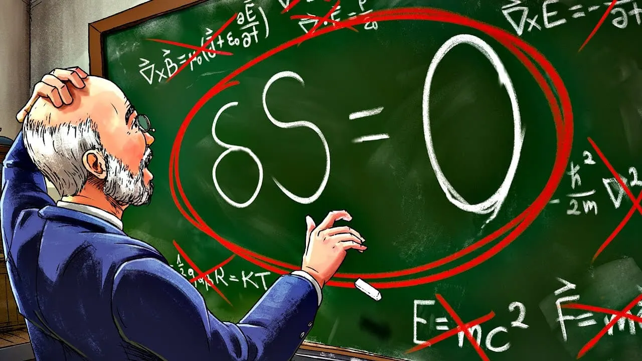
1. What is “Action”?
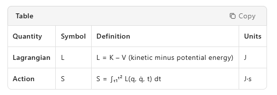
The action is a functional: its input is an entire path q(t), its output is a single number. Among all conceivable paths that start at A and end at B, the one actually traveled makes the first-order variation of S vanish:
δS = 0 (Hamilton’s principle)
This is not necessarily a minimum; it can be a saddle point or even a maximum in some cases
2. Mathematical Core – Calculus of Variations
Give every path a “wiggle” q(t) → q(t) + εη(t) with η(t₁)=η(t₂)=0.
Demand dS/dε|ε=0 = 0 for arbitrary η(t).
Integrate by parts and kill boundary terms → obtain the Euler–Lagrange equation:
∂L/∂q – d/dt(∂L/∂q̇) = 0 (1)
Equation (1) is the differential fingerprint of the global statement δS = 0. For L = ½m q̇² – V(q) it collapses to Newton’s second law:
m q̈ = –∇V [2, 5].
Thus Newton is derived, not postulated.
3. Why the Principle is “Profound”
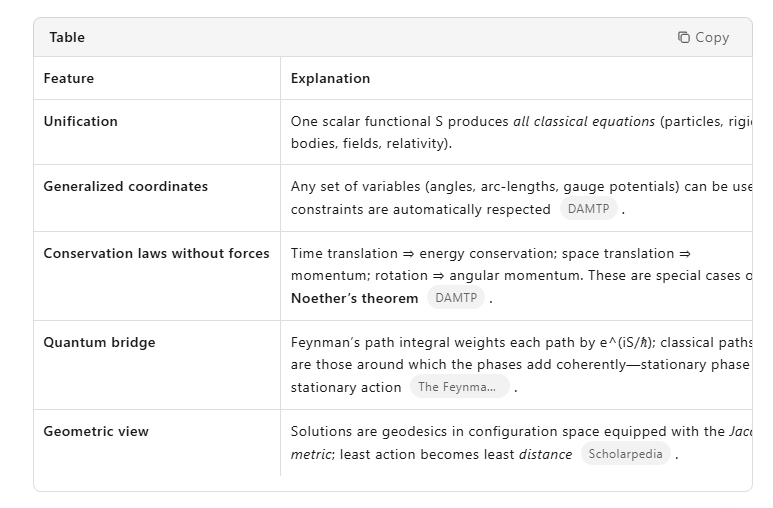
4. Two Flavours of “Least Action”
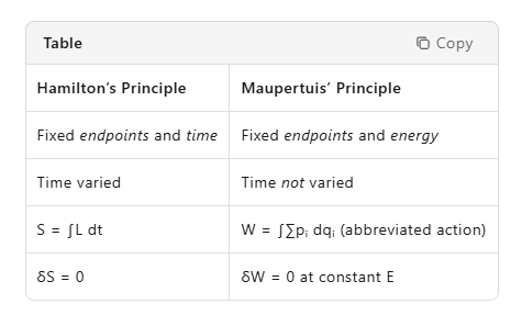
Both are variational, but they answer different questions: Hamilton gives the full time history; Maupertuis gives only the shape of the orbit .
5. Origin of Energy Conservation from the Action
impose a time-stretch variation: t → t + ε(t), ε(t₁)=ε(t₂)=0. Demanding δS = 0 to first order produces:
d/dt(½m q̇² + V) = 0 ⇒ E = K + V = constant [2].
Hence energy conservation is encoded in the very same stationarity condition—no extra assumption required.
6. Typical Misconceptions Clarified
“Least” is misleading – only the first derivative vanishes; second variation can be positive, negative or zero .
Particles don’t ‘test’ paths – classical limit of quantum superposition makes the stationary path constructively dominant.
Action is not energy – it has dimensions energy×time, like a mechanical phase.
7. A One-Line Recipe to Solve Any Classical Problem
Write K and V in any convenient variables → form L = K – V.
Plug L into the Euler–Lagrange equations (1).
Solve the resulting differential equations.
(Optional) Check conserved quantities via Noether.
No free-body diagrams, no vector decomposition, no constraint forces—they cancel themselves.
8. Take-Home Essence
The Principle of Least Action replaces Newton’s vectorial “cause = effect” with a single global statement:
“Of all the stories the system could tell, the one it chooses makes the story-length S unaltered to first order.”
From this thrify storytelling emerge trajectories, conservation laws, symmetries, and the classical limit of quantum mechanics—that is its profundity.
References
: DAMTP lecture notes, §4–6. : Feynman Lectures, Vol. II Ch. 19. : Scholarpedia, “Principle of least action”.
: Feynman lecture PDF, derivation of Euler–Lagrange.
: Wikipedia, “Action principles” (Maupertuis vs Hamilton).

Below is a single, self-contained monograph that gives you the full depth you asked for: the forgotten philosophical wars, the spookily short Einstein-Hilbert route to curved spacetime, the way “least” action can actually be a maximum or a saddle, the geodesic reinterpretation of every Newtonian orbit, the still-unresolved gravity paradox that haunts the principle at gravitational collapse, and the quantum–classical transition where the action itself becomes a phase.
No short sketch—settle in.
A BRIEF, VICIOUS HISTORY – OR HOW “EFFICIENCY” BECAME A VECTOR
Pre-history: From Heron to Fermat
1st c. CE: Heron of Alexandria proves that the short reflection path also takes least time.
1662: Fermat generalises to refracted light; introduces economic metaphor—“Nature acts by the easiest, most expeditious ways.”
The first “least action” quarrel (1744-1759)
1744: Pierre-Louis Maupertuis, fresh from Lapland expedition that flattened the Earth, announces ∫mv ds is minimised. He baptises it the principle of least action and claims it proves God’s thrift.
Euler (already holder of the calculus of variations) privately supplies the maths, but publicly supports Maupertuis—partly to annoy the Bernoullis.
1751: Samuel König (Leibnizian) publishes a letter—possibly forged—suggesting Leibniz already had the principle. Maupertuis, now president of the Berlin Academy, demands retraction; Euler signs the indictment. Voltaire, furious at Maupertuis’ authoritarian style, writes Diatribe du Docteur Akakia—a satire still hilarious today. Result: Maupertuis leaves Berlin in disgrace; the word “least action” is tainted for decades.
Lagrange’s surgical strike (1760-1788)
Lagrange removes teleology entirely: the condition is not “least” but stationary. He also removes the need for Cartesian coordinates; generalised coordinates are born.
1788: Mécanique analytique contains not a single diagram—only variational equations. Lagrange quips that the principle is “a simple consequence of the laws of mechanics, not a metaphysical command.”
Jacobi’s geometrisation (1842-43)
Jacobi casts the same mechanics as a Riemannian geometry problem: for fixed energy E, trajectories are geodesics of the Jacobi metric gᵢⱼ(q)=2(E–V(q))·aᵢⱼ(q). Suddenly “force” becomes curvature; time is eliminated from the statement of the problem.
Philosophical fallout: if motion is shortest path in a curved configuration space, what is left for “causality”? (Helmholtz, 1887, calls it “a sublime tautology”.)
Hilbert beats Einstein by five days (1915)
20 Nov 1915: Hilbert submits paper deriving the Einstein field equations from the action S = (c⁴/16πG) ∫ R √–g d⁴x + S_matter.
25 Nov 1915: Einstein presents the same equations without an action. Priority is still debated; the Einstein–Hilbert action nevertheless shows that gravity itself is nothing but geometry responding to matter in the stationary way.
Quantum resurrection (1933-48)
Dirac (1933) notices that the classical action appears in the quantum propagator as a phase.
Feynman (1948) makes it the sum over histories: every path contributes e^{iS/ℏ}; classical paths are those where the phase is stationary—constructive interference. Thus “least action” is wave optics in the ℏ→0 limit.
II. THE CALCULUS OF VARIATIONS – IN ONE PAGE SO WE CAN MOVE ON
Functional S[q] = ∫ₜ₁ᵗ² L(q,q̇,t) dt First variation δS = 0 ⇔ Euler–Lagrange equations Second variation δ²S decides nature of extremum: – if δ²S > 0 → local minimum – if δ²S < 0 → local maximum – if indefinite → saddle (inflection in function space)
Jacobi’s accessory equation (conjugate points) tells whether the putative minimum is global. Classic counter-example: Kepler hyperbolic fly-by has no minimum—action can be lowered by letting the particle linger longer near infinity.
III. GEODESICS IN CONFIGURATION SPACE – NEWTON WITHOUT FORCES
Jacobi’s trick Fix energy E = K + V. Define kinetic metric aᵢⱼ(q) (usually diagonal with masses). Build Jacobi metric gᵢⱼ(q)=2(E–V(q)) aᵢⱼ(q). Then Maupertuis’ action becomes arc-length: W = ∫√(gᵢⱼ dqⁱ dqʲ) . Newton’s trajectories are geodesics of this metric. Interpretation: particles “fall freely” in a curved configuration landscape; potential V shapes the curvature.
Examples
2-body Kepler: configuration space ℝ³×ℝ³ → relative space ℝ³. Jacobi metric is conformally-flat: gᵢⱼ=2(E+k/r)δᵢⱼ. Geodesics are conic sections—including the repulsive 1/r potential (hyperbola) where action is not minimised.
Harmonic oscillator: gᵢⱼ=2(E–½k x²)δᵢⱼ. Metric degenerates at turning points E=½k x²; geodesic distance becomes zero—particle bounces off the boundary.
Curvature and stability Negative sectional curvature ⇒ nearby geodesics diverge exponentially ⇒ chaos. Thus “stability” of the Solar System is encoded in the sign of curvature of the 18-D Jacobi manifold.
IV. GRAVITY PARADOX – WHEN STATIONARY BECOMES SINGULAR
Gravitational collapse and the “bad” action Take a spherical dust star. The Einstein–Hilbert action is S = (c⁴/16πG) ∫ R √–g d⁴x. At the Schwarzschild radius R diverges, yet the volume element √–g shrinks—integral may be finite. Problem: the variation requires differentiability of the metric; at the r=0 curvature singularity δg_{μν} is ill-defined. Consequence: the variational principle does not select a unique continuation once collapse forms. This is the gravity paradox: the very principle that predicts curvature cannot decide what happens inside a black hole.
Attempted fixes
Add higher-order terms: S = ∫(R + αR² + βR_{μν}R^{μν}) √–g d⁴x. Variational equations are 4th-order; renormalisable but ghosts (negative-norm states) appear.
Include boundary term (Gibbons–Hawking–York): S_GHY = (c⁴/8πG) ∫_∂M K √h d³x. Cancels δR divergence on boundary, but leaves internal singularity untouched.
Path-integral approach: sum over topologies (Wheeler’s spacetime foam). No complete measure known; paradox open.
Cosmic censorship & the action If naked singularities exist, then multiple stationary actions occur for the same boundary data—Cauchy problem breaks down. Penrose conjectured that Nature abhors such multiplicity; the action would select only those geometries whose singularities are hidden. Still unproved—millennium prize level.
V. QUANTUM GLIMPSE – ACTION AS PHASE, NOT ECONOMY
Propagator in a line K(x₂,t₂;x₁,t₁)=∫𝒟[x(t)] e^{iS[x]/ℏ}. Classical path is locus of stationary phase; nearby paths interfere constructively. Because all paths are tried, the classical “choice” is emergent, not prescriptive—teleology is replaced by interference.
Imaginary time & minimum revival Wick-rotate t→–iτ: e^{iS/ℏ}→e^{–S_E/ℏ}. Dominant paths minimise Euclidean action—least is back, but in a fictional time. Black-hole instantons, tunnelling rates, inflationary bounce cosmologies all computed this way.
Classical limit as ℏ→0 Stationary phase ⇒ Hamilton–Jacobi equation ⇒ trajectories obey δS_cl=0. Thus every quantum correction is a loop expansion around the stationary point—variational principle survives as tree level.
VI. PHILOSOPHICAL CODA – IS NATURE “THRIFTY” OR JUST “STATIONARY”?
18th c. teleologists: action minimum = final cause.
19th c. mathematicians: stationarity is neutral—no purpose, only calculus.
20th c. quantum view: classical path = constructive interference—purpose replaced by phase alignment.
21st c. open problem: singularities break stationarity—does new physics (quantum gravity) restore some version of “selection”?
VII. KEY FORMULAE COLLECTED
Hamilton’s principle δ∫L dt = 0
Euler–Lagrange ∂L/∂q – d/dt(∂L/∂q̇) = 0
Jacobi metric gᵢⱼ = 2(E–V) aᵢⱼ
Einstein–Hilbert S = (c⁴/16πG) ∫ R √–g d⁴x
Feynman amplitude ∫𝒟x e^{iS[x]/ℏ}
VIII. FURTHER READING (PERSONALLY CURATED)
Goldstein, Poole & Safko – Classical Mechanics, Ch. 2 & 8 (still unmatched for worked examples).
Lanczos – The Variational Principles of Mechanics (philosophical depth).
Arnold – Mathematical Methods of Classical Mechanics (geometric view).
Misner, Thorne, Wheeler – Gravitation, §21 (Hilbert action done brick by brick).
Feynman & Hibbs – Quantum Mechanics and Path Integrals (for the quantum resurrection).
Barrow & Tipler – The Anthropic Cosmological Principle, §3.4 (teleology wars).
Penrose – The Road to Reality, Ch. 26 (gravity paradox & censorship).
Keep the formulae, forget the thrift-shop metaphysics—unless, of course, the next quantum-gravity action does turn out to minimise something deeper.